Archive for the 'Microsoft Excel Tips' Category

Excel Tips and Tricks: How to Use the Excel Freeze Function

How frustrating is it when you scroll across a spreadsheet, and all the useful information disappears? Give your memory a break with the excel freeze function!

Excel Tips and Tricks: Freeze Function

Excel is an incredible tool for storing and managing data. However, scrolling across or down a spreadsheet is inevitable when dealing with magnitudes of cells. It would be ever so helpful to see the column and/or row titles while navigating other areas of the spreadsheet to make sense of and compare data.

BAM! In walks the Excel freeze function to save us all from repetitive strain injury.

Excel Freeze Function

So where can you find this handy tool?

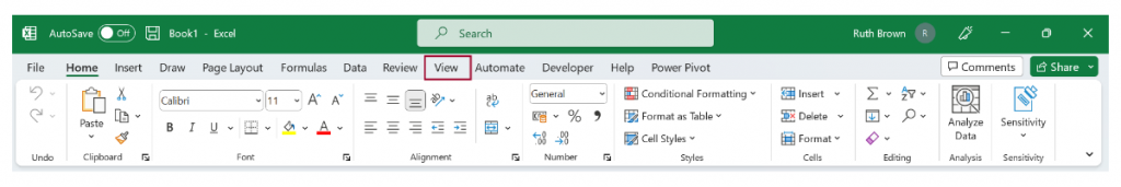
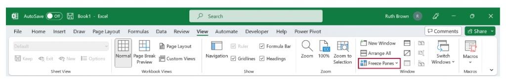
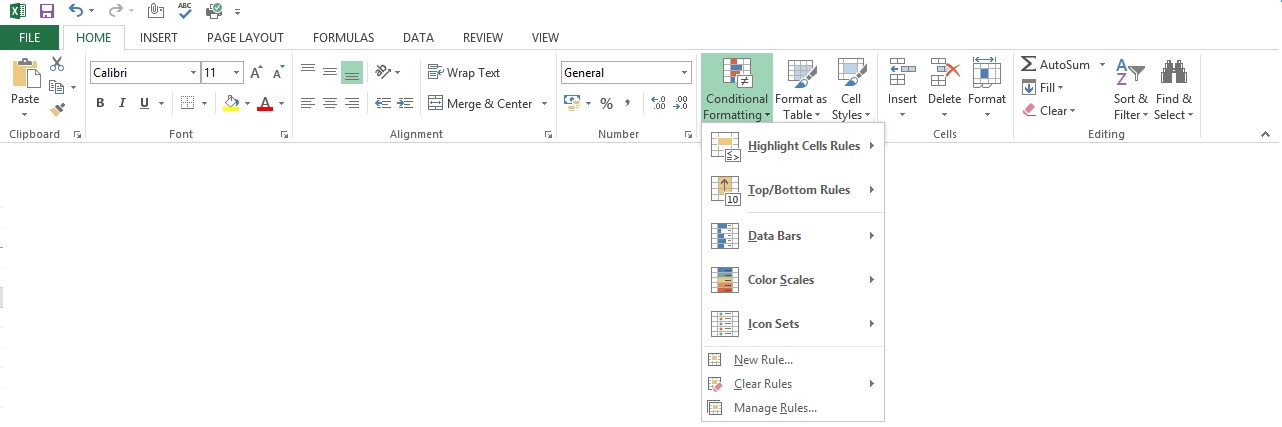
From the open spreadsheet, select the ‘View‘ tab and then the ‘Freeze Panes‘ function, which is found in the ‘Window’ group of the View tab (Select View > Freeze Panes).

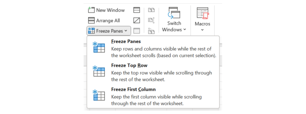
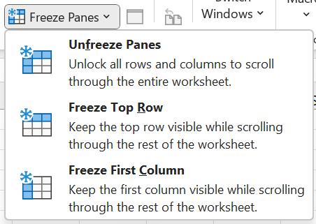
From here, you can see three options:

  1. Freeze Panes
  2. Freeze Top Row
  3. Freeze First Column
Step 1. Select View
Step 2. Select Freeze Panes
Freeze Pane Options

To get to grips with how to use the different Freeze options, check out the examples below!

1. Freeze Top Row

From freeze panes, select ‘freeze top row’.

Excel will automatically freeze the first row of the spreadsheet, which is indicated by a dark grey horizontal line beneath the first row.

2. Freeze First Column

From freeze panes, select ‘freeze first column’.

Again, Excel automatically freezes the first column of the spreadsheet, which is indicated by a dark grey vertical line to the right of the first column.

3. Freeze Panes

The above are extremely straightforward but don’t allow much flexibility. Freeze panes is slightly more complicated but gives more freedom.

For example, you can freeze multiple rows, multiple columns or multiple rows and columns. 

3.1 Freezing multiple rows

If you were looking to freeze a certain number of rows, select the row below the last row you want to remain visible and select freeze panes.

For example, if you want the first three rows to remain visible, select row four and freeze panes.

A dark grey horizontal line above row four and below row three indicates that these first three rows will remain visible whether you scroll up or down.

3.2 Freezing multiple columns

Freezing multiple columns is similar to the above example of freezing multiple rows.

Select the column to the right of the columns you want to remain visible and select freeze panes.

For example, if you want the first three columns to remain visible, select column four and freeze panes.

A dark grey vertical line to the left of column four and the right of column three indicates that these first three columns will remain visible whether you scroll left or right.

3.3 Freezing rows and columns

But what do we do when we want to freeze columns and rows?

Instead of selecting an entire row or column, we set one cell that controls which columns to the left and rows above are visible.

For example, if we want to freeze the first row and column, select the cell two rows down and two columns across (B2).

A dark grey vertical line to the left of the cell and a dark grey horizontal line above the cell indicates that the first row and column will remain visible whether we scroll across or down the spreadsheet.

4. Unfreeze Panes

After applying one of the three Freeze Pane options, the top Freeze Pane option will be replaced with ‘Unfreeze Panes‘. Simply select this to remove all columns and rows that have been frozen.

Unfreeze Panes

Thanks for reading, and we hope this helped! For more tips and tricks, check out our other blogs here!

Want more hands-on training? Infero also offers multiple Excel courses that will take you from beginner to pro. Get in touch for more information, book a course or receive a free consultation using the details below!

Suite 2556 37 Westminister Buildings Theatre Sqaure Nottingham
NG8 2EN

Why You SHOULD Learn New Skills In Excel

Now might be the time to get the new job you’ve always wanted. The Office of National Statistics reported in January that “The number of job vacancies in October to December 2021 rose to a new record of 1,247,000”. In some areas, however, things are still very competitive and it takes that little bit extra to stand out. 

One skill employers always look for proficiency in is MS Excel, because the software is extremely versatile and able to be turned to almost any task. It is also very widely used, in all types of industries including HR, Marketing, Retail and more. This is due to the depth of functionality that Excel has, being able to do everything from calculating, to sorting, organising and evaluating data, to providing business insights through easy to understand charts and visualisations. It is the default tool in almost every organisation, used by everyone from entry-level employees to senior staff.  

Whether you’re an employee trying to stand out from the crowd or an employer trying to raise productivity in your workplace, here are our top 5 reasons Excel should be your next step in education: 

Improving efficiency in the workplace 

Since Excel allows you to manipulate large amounts of data and even automate any data processing that takes place, it is easy to save hours of repetitive work. Tasks that take hours or days can be accomplished in minutes if you know how to access the correct tool in Excel. The greater your knowledge the more work that can be done speedily and efficiently, simply by accessing the sophisticated tools that Excel puts at your disposal. 

Knowledge of Excel will also help you stand out to prospective employers, or, perhaps, increase the appreciation that your present employer has for you, and give you a helping hand towards that promotion you are after. 

Takes the strain off the IT support 

In some organisations, where the workforce does not have a good knowledge of Excel, IT support may be required to help with ordinary, day to day work-tasks. This means that the individual may be unproductive whilst waiting for help from IT and the support staff’s time is taken up in solving an issue that wouldn’t even arise if the staff member had had some elementary training. Two staff members time are wasted on something trivial and very easily solvable. For both employees and employers, just a small amount of the right training is invaluable. 

Can Save the Company Money 

It might be that the company will at some point require someone with strong Excel skills. We live in an increasing data driven society, after all. At this point it would be far more cost effective for the employer to invest in their current staff. These are the people who have knowledge of, and commitment to, the company and could use that knowledge to uncover some money-making insights, if they only had the skills. Hiring someone already proficient in Excel will be time-consuming and costly. And it will take that person literally years to gain the knowledge and understanding of the business that current employees already have. Training is an investment of a few days that provides an excellent return in terms of workflow and productivity.  

Creates Higher Satisfaction for Employees 

Performing tasks in Excel without the proper training can mean that employees have a much higher workload than they really should, because they are not able to access the functionality contained in the programme. This, in turn, can lead to a team feeling unmotivated, with lower job satisfaction, even pressured and stressed because they may feel that they aren’t fully equipped for the task. Providing advanced Excel training for your team will increase both their motivation and productivity and your turnover. And, because they are being trained and valued, employee retention will be high.

Making Yourself Necessary 

The more efficient you become as a worker and the more time you save on the normal, everyday tasks, the more you will graduate to higher levels. Continuing your training to Excel advanced level can make you almost irreplaceable. Developing new skills helps you stay on top of your game and is a win-win for both the employee and the employer. 

If you’re looking for training for yourself or your employees, we offer Excel courses at three levels, catered for your pre-existing knowledge and experience.  

Excel Tip: Conditional Formatting

Conditional formatting is a feature within Microsoft Excel which is used for highlighting cells with a certain color, depending on the cell’s value. It can be a great tool for your Excel sheets, as it has various purposes and outcomes, whether you are after the top 5 values or a simple way to values that need your urgent attention.


To get to conditional formatting, go to the Home tab, then to the Styles command group:

conditional formating


There are plenty of in-built options for users who don’t want to modify anything or want to do things on the go. However, Excel gives users the chance to customize their own rules for conditional formatting for that added personal touch.


Conditional Formatting


To customize your own rules, follow the same steps above, select the New Rule command to bring the New Rule Dialogue Box.


Want to learn more? Check out our Courses and our other Hints and Tips


Microsoft Excel: Your Christmas List

Christmas is nearly upon us and we know how stressful it can be trying to budget and keep on track of finances. So here’s a helpful tip showing how you can use Microsoft Excel to plan ahead.


Using Excel create you Christmas List. The one below is from one of our staff:


Christmas List 1


Using “=SUM(D5:D11)” we have calculated the total cost that has been spent on the presents.  With a small budget of £100 we can also calculate what’s left to spend.


Now using the Filter function in the Data tab we can see what has been bought for each person. This works great if you have many presents like Santa.


Now when you click the down arrow next to “Who for?” we get the options below.

Christmas List 4


Below we can see what happens when “Mum” and “Blanks” are selected. Excel counted our calculations as a default but this can be changed. Right next to the Filter button used earlier is a smaller “Advanced” button. In there you can define your range. (So Mum has 3 presents)


Christmas List 7Christmas List 8


We hope you found this helpful. Look out for more tips on our blog Microsoft Excel Tips page and on twitter www.twitter.com/infero_training

Microsoft Excel VBA Tips: How to make a message box

Using Visual Basic of Applications can make your Excel workbooks a lot more user friendly and functional. In this blog post we will be looking how to create a message box in VBA for Excel 2007, 2010, and 2013.


The first message box we will be creating will be a small message box which shows the text “Hello World”. Before we can do this, we need to enable the developer tab on the ribbon. To do this you need to Click on File > Options > Customise Ribbon > and then check the developer tab like in the image below.

 How to make a message box 1


So on the developer tab; on the left hand side you can see a coding section. This is where you can easily access the Visual Basic Software, Macros and other options.


How to make a message box 2


Clicking the Visual Basic button will open up the Visual Basic Software. When making a message box, you are unable to record a macro to make this for you. You will need to type code to do it.


Here is what the Visual Basic Software looks like.


How to make a message box 3


To write some code we need to create a module to hold the code. To do this go to the top bar, click on Insert > Module


How to make a message box 4


Once you have done that you need then to create a Procedure to hold the Message Box.

Click Insert > Procedure > Type a name > Leave it set to Sub and Public > Click OK.

Note: The name cannot have a space in it.

How to make a message box 5


In the Coding window you can then type the following to create a message box


 How to make a message box 6


To run the Procedure/Macro, go back to your Excel window. This can be done by either closing the VBA window or just minimising it.


On the Developer tab > Click on Macros and the new HelloWorld Procedure/macro will be in here.


How to make a message box 7


Highlight the HelloWorld Macro and click run. You will get a little message appear with your message inside!


How to make a message box 8

Microsoft Excel Tips: Absolute Referencing

Absolute Referencing is a forgotten tool in your Toolbox called Excel. Daily you will probably find yourself using the fill handle on excel to automatically fill tables. This is called Relative Referencing and this will change the formula/function in a cell depending on which way you drag the cell.


So the example below we have a Product List at a made up computer company.Absolute Referencing 1


As you can see in the Total Quantity Price column I used the fill handle to drag my formula down the formula to the other rows to fill in the column. Because I dragged the fill handle down the numbers row numbers increased 1 at a time.
Absolute Referencing 2


Absolute Referencing allows us to lock a formula in a cell. Let’s see this in another example.


I’ve extended my table and added a Price After Tax column. This column uses the 20% (or 0.2) number in cell H1 to add the Tax onto the Price. Using the $ before both the H and the 1 you are able to “lock” this cell down. So when you use the fill handle the cell wont change.


Instead of typing the ‘$’ in the formula you could press the F4 key on your keyboard to automatically add the ‘$’ to that cell reference.

Microsoft Excel Tips: How to Personalize your Table

When you use Excel the table can look really boring and plain; however in the newer versions (2007 and

Microsoft Excel 2007 Cell Styles Menu

2010) you are able to customize your tables by using different font styles and colours as well. There are also different shades of colour and sizes of text you can use. To change you table here’s how to do it:


  1. Click on the Cell Styles link on the toolbar
  2. This will give you a list of all the different styles that are available to you when making your table
  3. Click on the cell you want to personalize and then choose the style you want.


Want more tips; just visit our Microsoft Excel Tips page